Summary
In 2023, Kentucky had the fifth-largest drug overdose fatality rate in the United States, and 79% of those deaths involved opioids. To help combat the opioid epidemic in Kentucky, CAAI works with the Rapid Actionable Data for Opioid Response in KY (RADOR-KY) team to provide support with machine learning (ML) techniques. Overall, the team works to create a statewide surveillance system to monitor and respond to the opioid crisis, collecting data from a variety of sources and agencies around Kentucky. One key part of the project is predictive analytics, using ML techniques to forecast future trends of opioid overdoses in different areas of Kentucky. The goal is to provide accurate forecasts based on different geographical levels to identify which areas of the state are likely to be the most “high risk” in future weeks or months. These forecasts are then made available to relevant stakeholders through a dashboard website. With this information, adequate support can be prepared and provided to those areas with the hope of treating victims in time and reducing the number of deaths associated with opioid-related incidents.

Datasets/Models
Data Pre-Processing
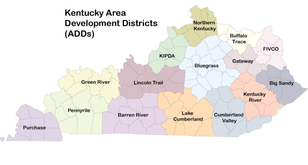
The first step was to analyze what geographical level would be most appropriate for building and training a forecasting model. The data we use to track suspected opioid overdose incidents comes from Kentucky Emergency Medical Services (EMS) responses, beginning in January 2018 and continually updated weekly. With this data, we could group incidents based on many different geographical levels: state, Area Development District (ADD), county, zip code, tract, block group, and block. Through experimentation, it seemed that the county level was likely the most appropriate scale. The state level is too broad for useful results, while any level smaller than the county level proved to be too sparse. Smaller geographical levels contain too few positive examples of incidents for any model to successfully learn the trends of each area. However, data sparsity remains a problem even at the county level in less-populated areas, so we have also worked with ADDs, which are larger groupings of counties. Additionally, the temporal level was chosen to be at the monthly scale, rather than yearly or weekly, due to early testing results suggesting the best performance at monthly levels.
Additional Data
Time-series forecasting models typically are able to use previous values of the target series to determine the trends and patterns that they use to predict into the future. However, many models can also use additional data sources to aid in the predictions, called covariates. A variety of data from different sources has been tested as covariates, including:
- Social determinants of health for each county, such as unemployment rate, vehicle access, and age distributions
- Aggregated Medicaid claims containing counts of individuals receiving medication for Opioid Use Disorder (OUD) or behavioral health treatment
- Kentucky State Police drug seizures for opioid substances
- Kentucky Department of Corrections’ substance use risk measures for supervision intakes and releases
- Syndromic surveillance-detected nonfatal overdose emergency department visits
- EMS incidents from other nearby regions
- Monthly temperature and precipitation values
Some covariates, such as weather, are future covariates, meaning that their values are known into the future and can be used at prediction time. Others, such as drug seizures, are past covariates, so their historical data can be used to capture trends and correlations, but future values are not known ahead of time. The social determinants of health are an example of a static covariate, meaning the value is not expected to change significantly over time, but it can still be used to distinguish between the characteristics of different areas.
Training
Several different models have been evaluated for forecasting. First, Linear Regression is the simplest and most general model, but it can be applied to time series forecasting as well. Second, the N-Linear model is a simple, one-layer neural network built specifically for time series forecasting. Finally, the Temporal Fusion Transformer (TFT) is a large deep learning architecture, also built for forecasting. This is the most complex model evaluated here, using multiple layers and a self-attention mechanism to weight the importance of data at different time steps. These models were chosen among many others for two primary reasons. First, they can support all types of covariates, including future, past, and static. Many other models, particularly statistical methods, can only utilize future covariates when making predictions. Second, these models possess multivariate capabilities, allowing for separate series, such as each county or ADD, to be trained and evaluated with one model. That way, the model can learn the overall trends that each region shares, while also picking up on exclusive patterns specific to each region.
Before training, pre-processing techniques were performed to normalize each grouping’s data to its own mean and address missing values. Normalization is required because many of the regions have vastly different scales when counting opioid overdoses, and normalizing these ensures that the model considers all regions equally. Addressing missing values is required because many of the data sources for the covariates have misaligned data availability time frames. These missing values were filled using a simple Exponential Smoothing model to predict timestamps for which data was missing. For each variable, an additional binary flag was created to indicate whether the data was originally missing.
When training, we have tested a variety of configurations of models and covariates to determine the most effective methods for creating accurate predictions. To do this, each model is evaluated separately, as well as each covariate. Two primary methods of training have been used as well. The first is a standard training/testing split, where the model is trained on 90% of the entire series at once and produces predictions for the last 10% or so. This is smaller than the standard 20% testing size, and it was chosen to reflect real-world capabilities and use cases. Predictions made for more than a few months out are not practical or useful, so we limited the size of the test set. However, a more thorough evaluation can be achieved through the second training method using an expanding window. In this technique, the model is initially trained on the first two years of data and produces predictions for the next three months. Then, the next three months of real data are incorporated, and the model is refit, learning from the error in its predictions. It can then predict for the next three months, and this pattern continues until all data has been used for training. This method is more thorough than the standard training/testing split and allows for a more complete evaluation of performance.
Results
Each run was evaluated with the Root Mean Squared Error (RMSE), which is a common performance metric for time-series forecasting. Because it is a measure of prediction error, a lower value is better. First, comparisons are made between each model, training type, and geographical grouping (county, ADD, state).
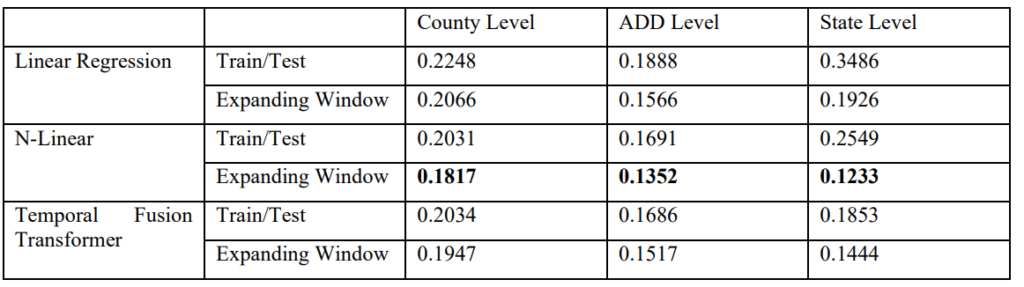
In all cases, the expanding window method achieved better performance over the same test period as the standard train/test split. Additionally, the N-Linear model performed the best overall. Comparisons between groupings show that performance is generally best at the ADD level, where sparsity is less of an issue compared to the county level.
Each covariate was also tested independently to determine its impact. Overall, the best performing covariates are the Medicaid data for OUD treatment, DOC intake/release data, and a covariate called Nearby Trends that, for each county, averages the EMS suspected opioid overdose trends of other counties in the same region.
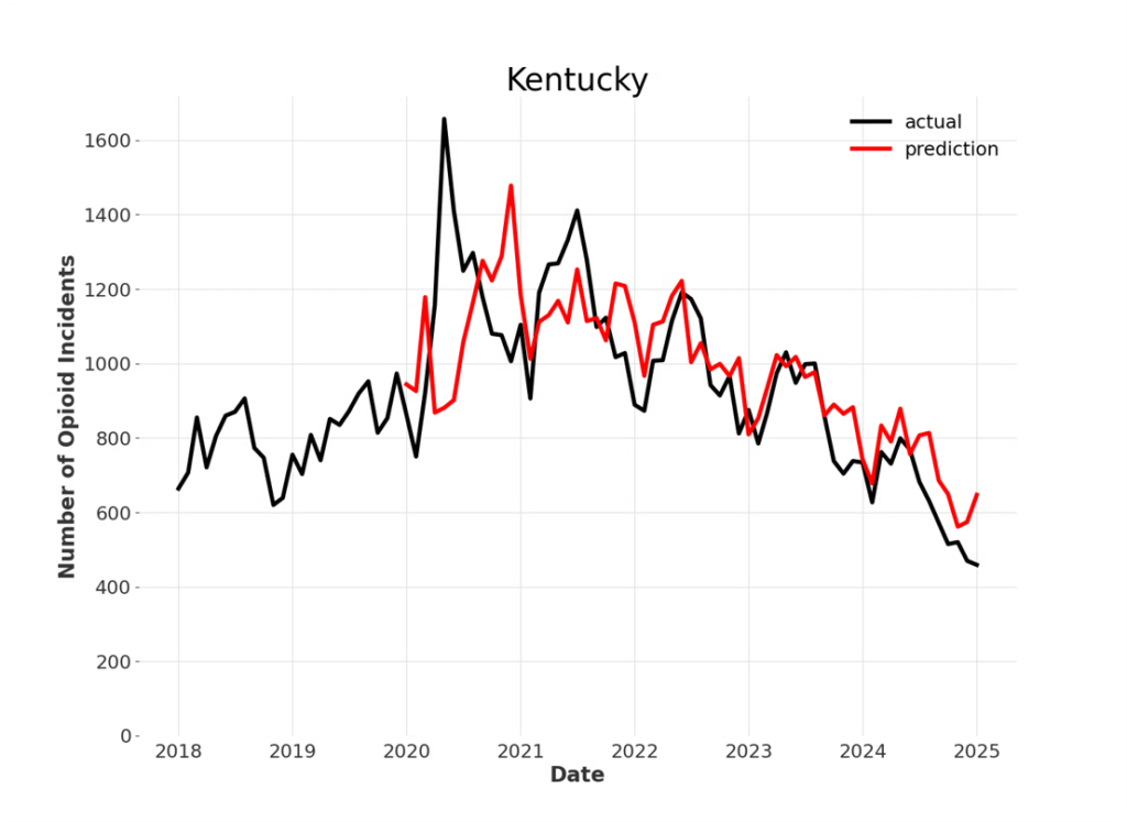
An example of performance for statewide predictions is shown below. With the expanding window method, predictions can be generated throughout the series, and it is clear that as the model uses more data over time, it produces more accurate forecasts.
We will continue to test new models and external data sources to improve forecasting accuracy. Still, the current results show that forecasting opioid overdoses around Kentucky is possible with limited error and will prove useful to state agencies for determining when and where opioid overdoses can be expected to increase or decrease.
Access
The dashboard site that displays these predictions, among other data, can be found on the RADOR-KY website.
Ownership
A presentation covering this topic was given at UK’s AI/ML seminar on 10/17/2024.
RADOR was presented at the American Public Health Association’s Annual Meeting & Expo 2024.
Implementation and Assessment of Machine Learning Models for Forecasting Suspected Opioid Overdoses in Emergency Medical Services Data, a paper written about this topic, was accepted to the 2025 AMIA Symposium.
This research was supported in part by the National Institutes of Health under award numbers R01DA057605-01, R01DA057605-01S1, and R01DA057605-01S2. The content is solely the responsibility of the authors and does not necessarily represent the official views of the NIH.
Resources
Aaron Mullen has been working on RADOR for two years, at first being funded 20% of his time. As of August 2025, Aaron is funded 50%.